Reinforcement Learning [Part 2]
Recap
In the previous post we introduced state-value and history-value functions for a policy $\pi$ which allow us to compute the expected return at different starting points in time. They can be used to compare the effectiveness of different policies, which plays well with our intent of finding the optimal policy for the task at hand.
How do we compute them?
We derived a generalized form of the Bellman equation which, under a set of stronger hypotheses on the agent and on the environment, simplifies to a manageable expression which we feel confident to solve.
It remains to prove that those stronger hypotheses are reasonable and that they do not damage our chances of finding the overall optimal policy.
This will be our focus for today.
Decision rules: a breakdown
We introduced decision rules as mappings between $\mathcal{H}_t$, the set of possible histories of our system up to time $t$, and $\mathcal{P}(\mathcal{A})$, the collection of probability distributions over the set of actions:
$$\begin{equation} d_t: \mathcal{H}_t \to \mathcal{P}(\mathcal{A}) \end{equation}$$
This definition provides the greatest amount of generality and flexibility - we usually refer to this class of decision rules as history-dependent randomized decision rules: every action and event up to the current time instant is taken into account before specifying the agent preferences for the next action.
This class of decision rules will be denoted by $D^{HR}_t$.
Everything comes with a price: it is computationally very expensive to keep track of a function whose input dimension grows exponentially in time.
Consider, for example, a state space $\mathcal{S}$ with five elements equipped with an action set $\mathcal{A}$ composed of three choices.
For $t=1$ we have 5 elements in $\mathcal{H}_1$ (we take $t=1$ as starting state).
For $t=2$ we have 5x3x5=75 elements in $\mathcal{H}_2$.
For an arbitrary $t\in\mathbb{N}$ we have
$$\begin{equation} |\mathcal{H}_t| = 5^t 3^{t-1} \end{equation}$$
which, you surely agree with me, is going to become problematic soon enough, even if the system is ridiculously small.
A much more convenient class of decision rules is the collection of randomized markovian decision rules, which we denote by $D^{MR}$: the action choice is chosen randomly from a probability distribution depending only on the current state of the system (no $t$ subscript this time!).
This can be stated formally saying that every $d\in D^{MR}$ if a function from $\mathcal{S}$ to $\mathcal{P}(\mathcal{A})$.
The computational gain is evident: a markovian randomized decision rule $d$ only requires $|\mathcal{S}||\mathcal{A}|$ memory slots - a much more feasible choice.
Policies: a breakdown
To each class of decision rules we can associate a class of policies:
$\pi$is a history-dependent randomized policy if$$\begin{equation} \pi = (d_1, \, d_2, \, \dots) \quad \quad \text{where } d_i\in D^{HR}_i \end{equation}$$We shall refer to this class using$\Pi^{HR}$;$\pi$is a markovian randomized policy if$$\begin{equation} \pi = (d_1, \, d_2, \, \dots) \quad \quad \text{where } d_i\in D^{MR} \end{equation}$$We shall refer to this class using$\Pi^{MR}$.
Markovian randomized decision rules are a subset of history-dependent randomized decision rules, which implies that
$$\begin{equation} \Pi^{MR} \subset \Pi^{HR} \end{equation}$$
Before proceeding anything further is time to give a proper definition of optimal policy.
Optimal policies
Using the concept of state-value function we can affirm that a policy $\pi$ is better than a policy $\pi'$ if
$$\begin{equation} v^1_\pi(s) \geq v^1_{\pi'}(s) \quad \forall s\in\mathcal{S} \end{equation}$$
where $s$ is the initial state of our system.
A policy $\pi$ is said to be optimal if
$$\begin{equation} v^1_\pi(s) \geq v^1_{\pi'}(s) \quad \forall s\in\mathcal{S} \end{equation}$$
for all $\pi'\in\Pi^{HR}$ [remember that randomized history-dependent policies are the most general class!].
It is important to remark that $v_{(\cdot)}$ is an expected value - even if a policy $\pi$ is better on average than a policy $\pi'$ it might still happen than an experiment using policy $\pi$ produces a higher return compared to an experiment using policy $\pi'$: stochasticity baby!
We can now ask the following question: are we compromising our search for an optimal policy if we restrict our attention to markovian randomized policies?
In other words, are we going to achieve a lower expected return if we focus on policies which do not use the whole system history before committing to an action?
It depends on the environment - we shall see why.
Return: a different viewpoint
Let's recall the definition of state-value function for a policy $\pi$:
$$\begin{equation} \begin{split} v_\pi^1(s_1) &:= \mathbb{E}[G_1 \,|\, S_1=s_1] = \\ &= \sum_{i=1}^{T} \gamma^{i-1}\, \mathbb{E}[R_{i+1}\,|\, S_1=s_1] \end{split} \end{equation}$$
where $s_1\in\mathcal{S}$, $\,\gamma\in[0, 1)$ and $T\in\mathbb{N}\cup\{+\infty\}$.
Using the definition of expectation we get:
$$\begin{equation} v_\pi^1(s_1) := \sum_{i=1}^{T} \gamma^{i-1}\, \sum_r r \, \mathbb{P}(R_{i+1}=r\,|\, S_1=s_1) \end{equation}$$
which can be decomposed using the law of total probability
$$ \begin{equation}\label{return-general} v_\pi^1(s_1) := \sum_{i=1}^{T} \gamma^{i-1}\, \sum_r r \, \sum_{s\in\mathcal{S}} \sum_{a\in\mathcal{A}} \mathbb{P}(R_{i+1}=r\,|\, A_t=a, S_t=s, S_1=s_1) \, \mathbb{P}(A_t=a, S_t=s \,|\, S_1=s_1) \end{equation} $$
This is were we need to introduce the first additional hypothesis on the environment: let's suppose that rewards are markovian. Then
$$\begin{equation} \mathbb{P}(R_{i+1}=r\,|\, A_t=a, S_t=s, S_1=s_1) = \mathbb{P}(R_{i+1}=r\,|\, A_t=a, S_t=s) \end{equation}$$
which can be plugged in equation \ref{return-general} to get
$$\begin{equation}\label{return} v_\pi^1(s_1) := \sum_{i=1}^{T} \gamma^{i-1}\, \sum_r r \, \sum_{s\in\mathcal{S}} \sum_{a\in\mathcal{A}} \underbrace{\mathbb{P}(R_{i+1}=r\,|\, A_t=a, S_t=s)}_{\text{environment}} \, \underbrace{\mathbb{P}(A_t=a, S_t=s \,|\, S_1=s_1)}_{\pi\text{-dependent}} \end{equation}$$
We have isolated the part of the equation which depends on the policy $\pi$ - to enforce this concept let's mark it with a superscript:
$$\begin{equation} \mathbb{P}^\pi(A_t=a, S_t=s \,|\, S_1=s_1) \end{equation}$$
History is overrated
Now, suppose that the following holds:
$\textbf{Theorem 1}$ - For each history-dependent randomized policy $\pi$ and for each $s_1\in\mathcal{S}$ there exists a markovian randomized policy $\tau$ such that
$$\begin{equation} \mathbb{P}^\pi(A_t=a, S_t=s \,|\, S_1=s_1) = \mathbb{P}^\tau(A_t=a, S_t=s \,|\, S_1=s_1) \end{equation}$$
for every $t\in\{1, 2, \dots\}$, for every $a\in\mathcal{A}$ and for every $s\in\mathcal{S}$.
Using equation \ref{return} it would follow that `$$ \begin{equation} v^1_\pi(s_1) = v^1_\tau(s_1) \end{equation} $$` which can be used to show that an optimal policy in the class of markovian randomized policies is just as good as an optimal policy in the class of history-dependent randomized policies!
It is strikingly easy: let $\pi^*$ be an optimal policy in $\Pi^{HR}$ and let $\tau^*$ be an optimal policy in $\Pi^{MR}$.
We know that $\Pi^{MR}\subset\Pi^{HR}$ which implies that
$$\begin{equation} v^1_{\pi^*}(s) \geq v^1_{\tau^*}(s) \quad \quad \text{for every } s\in\mathcal{S} \end{equation}$$
Nonetheless, for every $s\in\mathcal{S}$ there exists a policy $\alpha_{s}$ in $\Pi^{MR}$ such that
$$\begin{equation} v^1_{\pi^*}(s) = v^1_{\alpha_{s}}(s) \end{equation}$$
But $\tau^*$ is optimal in $\Pi^{MR}$:
$$ \begin{align} v^1_{\tau^*}(s) \geq v^1_{\alpha_{s}}(s) &= v^1_{\pi^*}(s)\geq v^1_{\tau^*}(s) \quad \quad \text{for every } s\in\mathcal{S} \\\\ \Rightarrow \quad v^1_{\pi^*}(s) &= v^1_{\tau^*}(s) \quad \quad \text{for every } s\in\mathcal{S} \end{align} $$
We have thus proved that if the environment is markovian and Theorem 1 holds it is sufficient to search for an optimal policy in the class of markovian randomized policies $\Pi^{MR}$.
The proof of Theorem 1 is not difficult and proceeds by induction - it can be found on Peterman's book as Theorem 5.5.1.
Interlude

Let's pause for a second to summarize what we have achieved and what we are still missing
We defined the concept of optimal policy as well as providing an extremely useful result to restrict the number of candidates for optimality.
Nonetheless we have not found yet an equation which gives us directly the optimal policy as a solution - we have no other way to find it, at the moment, than evaluating the state-value function of each policy in $\Pi^{MR}$.
Sadly, $\Pi^{MR}$ is an infinite set, which means that we cannot find the optimal policy using brute force.
What now?
Sometimes it is better to simplify and understand the matter at hand in a smaller context before facing the original more complex issue.
In our case, we are going to study a reinforcement learning problem with fixed and finite time-horizon $T$ - not a random variable, but a natural number which does change between different simulation of our agent.
We shall derive a set of equations called optimality equations whose solution, unsurprisingly, is an optimal policy in this simplified setting.
The form of the equation will suggest us a more general formulation which can be used as an optimality equation for problems with arbitrary and random time-horizon $T$, the ones we are genuinely interested in.
Let's do it!

Optimality for fixed & finite time-horizons
Suppose, as we just suggested, that $T$ is a fixed and finite natural number.
This means that $S_T$ is the terminal state of our agent: no actions to be taken once we reach that point.
We assume that there exists a terminal reward function, $r_T:\mathcal{S}\to\mathbb{R}$: if $S_T=s$ is the terminal state of the simulation then the agent receives a reward equal to $r_T(s)$.
We proved that a policy $\pi$ is optimal if $v_{\pi}^1(s)\geq v_{\alpha}^1(s)$ for all $\alpha\in\Pi^{MR}$ and for all $s\in\mathcal{S}$.
Define
$$\begin{equation}\label{optimal_naive_sup} v^t_* (s_t) := \sup_{\pi\in\Pi^{MR}} v^t_\pi (s_t) \quad \forall s_t \in\mathcal{S} \end{equation}$$
for every $t\in\{1, 2, \dots, T\}$.
It follows that $v^1_*$ is a function (not a policy, be careful!) which satisfies
$$\begin{equation} v_{*}^1(s)\geq v_{\alpha}^1(s) \quad \quad \forall\,\alpha\in\Pi^{MR}\, , \, \forall \, s\in\mathcal{S} \end{equation}$$
Even though equation $\ref{optimal_naive_sup}$ is pretty straight-forward it does not provide, by itself, a way to actually compute $v^t_*$.
Luckily enough, it can be proved (Puterman - Th. 4.3.2) that $\{v^t_*\}_{t=1}^T$ are a solution of the following system of equations:
$$\begin{equation}\begin{split} &\forall t\in\{1,\dots, T-1\}: \\\\ &v^t_*(s_t) = \max_{a\in\mathcal{A}}\bigg\\{\mathbb{E}\left[R_{t+1}\:|\:A_t=a,\: S_t=s_t\right] + \sum_{s\in\mathcal{S}} v^{t+1}_*(s) \\: \mathbb{P}(S_{t+1} = s\:|\: A_{t}=a, \\, S_t = s_t)\bigg\\} \\\\ &v^T_*(s_T) = r_T(s_T) \end{split}\label{optimality-finite}\end{equation}$$
where we have implictly assumed that state transitions are markovian, i.e.
$$\begin{equation} \mathbb{P}(S_{t+1} = s\:|\: A_{t}=a, \, S_t = s_t) = \mathbb{P}(S_{t+1} = s\:|\: A_{t}=a, \, H_t = h_t) \end{equation}$$
We have used a $\max$ over $\mathcal{A}$ because we are also assuming that the set of possible actions is finite.
Equations \ref{optimality-finite} are usually referred as optimality equations.
We shall see that they can be used to actually compute $v^t_*$, which for the moment stands as an upper-bound on the corresponding function for our hypothetical optimal policies. If we could prove that there exists a policy $\pi^*$ such that
$$\begin{equation} v^t_*(s_t) = v^t_{\pi^*}(s_t) \quad\quad \forall s_t\in\mathcal{S} \end{equation}$$
then we would be a good deal closer to the solution of the optimality problem for finite and fixed time-horizon systems.
Puterman comes in our aid once again, with Theorem 4.3.3 (which slightly generalize).
Theorem 4.3.3 - Let $\{v^t_*\}_{t=1}^T$ be a solution of the optimality equations and suppose that $\pi^*=(d_1^*, \dots, d_{T-1}^*)\in\Pi^{MR}$ satisfies
$$\begin{split} &\mathbb{E}_{\pi^*}\left[R_{t+1}\:|\:S_t=s_t\right] + \sum_{s\in\mathcal{S}, \, a\in\mathcal{A}} v^{t+1}_{\pi^*}(s) \: b_{d_t^*(s_t)}(a)\: \mathbb{P}(S_{t+1} = s\:|\: A_{t}=a, \, S_t = s_t) = \\\\ &\quad\quad = \max_{a\in\mathcal{A}}\bigg\\{ \mathbb{E}\left[R_{t+1}\:|\:A_t=a,\: S_t=s_t\right] + \sum_{s\in\mathcal{S}} v^{t+1}_*(s) \: \mathbb{P}(S_{t+1} = s\:|\: A_{t}=a, \, S_t = s_t)\bigg\\} \end{split}\label{trial}$$
for $t\in\{1,\dots,T\}$. Then
$$\begin{equation} v^t_*(s_t) = v^t_{\pi^*}(s_t) \quad \quad \forall s_t \in\mathcal{S}, \: \forall t\in\{1,\dots,T\} \end{equation}$$
which implies that $\pi^*$ is an optimal policy.
We can actually say something more.
Let's rewrite \ref{trial} in a slightly different but equivalent way:
$$\begin{equation}\begin{split} &\sum_{a\in\mathcal{A}}\: b_{d_t^*(s_t)}(a) \, \bigg\\{\mathbb{E}_{\pi^*}\left[R_{t+1}\:|\:A_t=a, S_t=s_t\right] + \sum_{s\in\mathcal{S}} v^{t+1}_{\pi^*}(s) \: \mathbb{P}(S_{t+1} = s\:|\: A_{t}=a, \, S_t = s_t) \bigg\\} = \\\\ &\quad\quad = \max_{a\in\mathcal{A}}\bigg\\{\mathbb{E}\left[R_{t+1}\:|\:A_t=a,\: S_t=s_t\right] + \sum_{s\in\mathcal{S}} v^{t+1}_*(s) \: \mathbb{P}(S_{t+1} = s\:|\: A_{t}=a, \, S_t = s_t)\bigg\\} \end{split}\label{trial-2} \end{equation}$$
But a very simple calculus lemma stays the following:
Lemma - Let $\{w_i\}_{i\in I}$ be a finite collection of real numbers and let $\{q_i\}_{i\in I}$ be a probability distribution over $I$ (i.e. $q_i\in[0,1]$ and $\sum_i q_i=1$); then
$$\begin{equation} \max_{i\in I} w_i \geq \sum_{i\in I} q_i w_i \end{equation}$$
Equality holds if and only if
$$\begin{equation} q_i = 0 \end{equation}$$
for every $i$ such that $w_i < \max_{i\in I} w_i$.
In our case $\{w_i\}_{i\in I}=\mathcal{A}$ and $b_{d_t^*}(\cdot)$ is our probability distribution, which implies that a policy $\pi^*=(d_1^*, \dots, d_{T-1}^*)$ is optimal if and only if it chooses with positive probability only those actions which maximize the right hand side of equation \ref{optimality-finite}.
In other words, solving the system of optimality equations provides us with the optimal actions to be taken at each step of our reinforcement learning problem, which in turn completely determine the set of optimal policies (which can even be chosen to be deterministic, instead of randomized!).
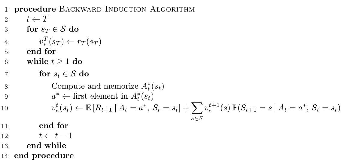
Solving equations \ref{optimality-finite} is not so difficult, considering that we are assuming that $\mathcal{A}$ is finite: a possible recipe is given by the Backward Induction Algorithm.
It determines
$$\begin{equation} A^*_t(s_t):= \underset{a\in\mathcal{A}}{\mathrm{argmax}} \bigg\\{\mathbb{E}\left[R_{t+1}\:|\:S_t=s_t,\: A_t=a\right] + \sum_{s\in\mathcal{S}} v^{t+1}_*(s_t, s, a) \: \mathbb{P}(S_{t+1} = s\:|\: A_{t}=a, \, S_t = s_t)\bigg\\} \end{equation}$$
for all $t\in\{1,\dots, T-1\}$ and $s_t\in\mathcal{S}$ - i.e. the set of actions which maximize the expression in curly brackets.
Here is the pseudo-code:
Optimality equations for an arbitrary time-horizon
We have seen that the solution of
$$\begin{equation}\begin{split} &\forall t\in\{1,\dots, T-1\}, \: \forall s\in \mathcal{S}: \\\\ &v^t_*(s) = \max_{a\in\mathcal{A}}\bigg\\{\mathbb{E}\left[R_{t+1}\:|\:A_t=a,\: S_t=s\right] + \sum_{s'\in\mathcal{S}} v^{t+1}_*(s') \: \mathbb{P}(S_{t+1} = s'\:|\: A_{t}=a, \, S_t = s)\bigg\\} \\\\ &v^T_*(s) = r_T(s) \end{split}\end{equation}$$
provides us with the state-value function of an optimal policy (as well as the policy itself!) if the time-horizon is fixed and finite.
Is there a way to reformulate this system to accomodate the general case - where $T$ is a random variable, potentially finite?
So far we have supposed that rewards and state transition probabilities were markovian. We want to make two more assumptions on the environment:
- rewards are stationary:
$$\begin{equation} \mathbb{E}\left[R_{t+1}\:|\:A_t=a,\: S_t=s\right] = \mathbb{E}\left[R_{j+1}\:|\:A_j=a,\: S_j=s\right] \end{equation}$$for every$t, j\in\{1, \dots, T-1\}$; - state transition probabilities are stationary:
$$\begin{equation} \mathbb{P}\left(S_{t+1}=s' \:|\:A_t=a,\: S_t=s\right) = \mathbb{P}\left(S_{j+1}=s' \:|\:A_j=a,\: S_j=s\right) \end{equation}$$for every$t, j\in\{1, \dots, T-1\}$.
It make sense, then, to define:
$$\begin{align} r(a, s) &:= \mathbb{E}\left[R_{2}\:|\:A_1=a,\: S_1=s\right] \\\\ p(s'\,|\, a, s)&:=\mathbb{P}\left(S_{t+1}=s' \:|\:A_t=a,\: S_t=s\right) \end{align}$$
which can plugged into the optimality equations leading to:
$$\begin{equation}\begin{split} &\forall t\in\{1,\dots, T-1\}, \: \forall s\in \mathcal{S}: \\\\ &v^t_*(s) = \max_{a\in\mathcal{A}}\bigg\\{r(a, s) + \sum_{s'\in\mathcal{S}} v^{t+1}_*(s') \: p(s'\,|\, a, s)\bigg\\} \\\\ &v^T_*(s) = r_T(s) \end{split}\end{equation}$$
What would happen if we were to pass to the limit now, for $t\to +\infty$?
The only terms depending on $t$ in the first equation are $v^t_*$ and $v^{t+1}$, thanks to our stationarity assumption.
If the sequence $\{v^{t}\}_t$ (which is infinite, if $T=\infty$) converged to a proper limit $v_*$ for $t\to +\infty$ we would find that
$$\begin{equation} v_*(s) = \max_{a\in\mathcal{A}}\bigg\\{r(a, s) + \sum_{s'\in\mathcal{S}} v_*(s') \: p(s'\,|\, a, s)\bigg\\} \\\\ \end{equation}\label{bellman-optimal}$$
Equation \ref{bellman-optimal} is called Bellman optimality equation and it does actually provide us with an optimal state-value function in the general case.
But this will be topic of the next episode.